Results (post-processing)

Parameter estimation results

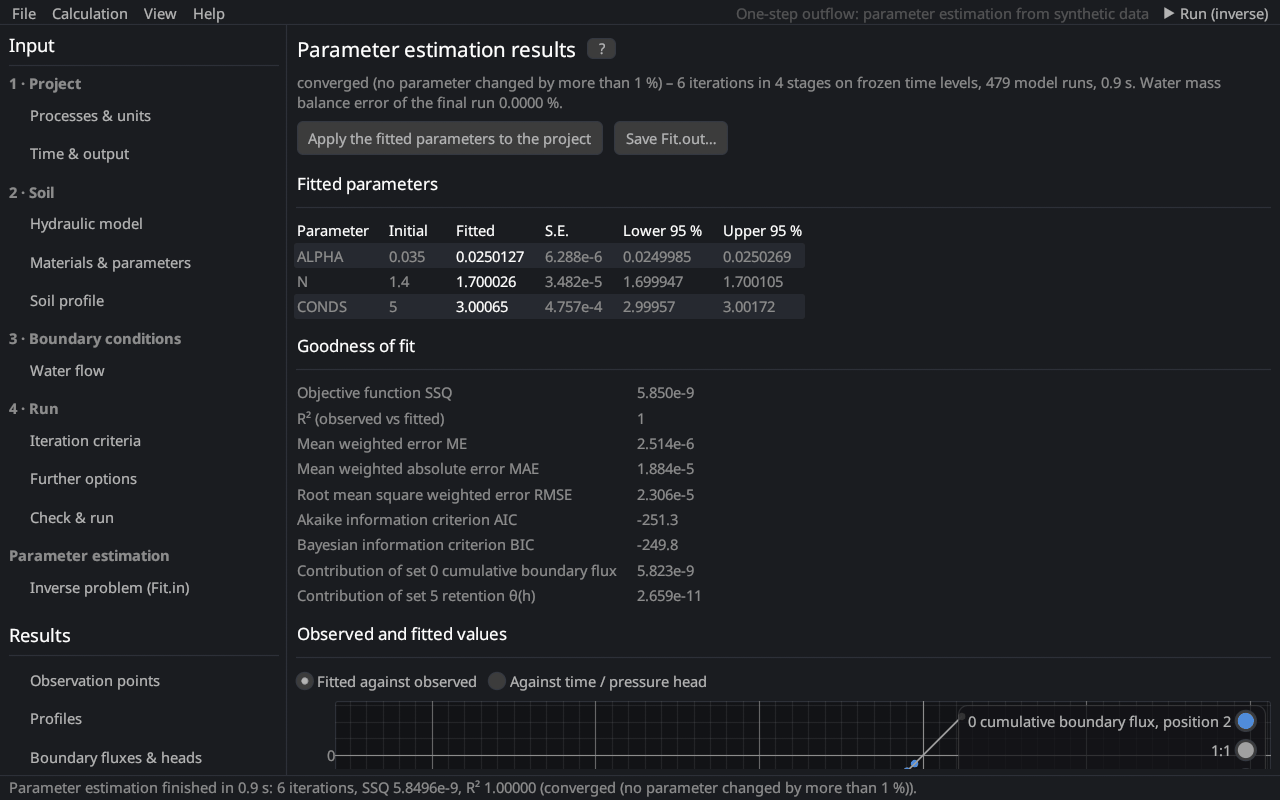
The page shows the run and the results of a parameter estimation, the content of Fit.out of HYDRUS-1D (Inverse Solution Information).

The results page Parameter estimation with the fitted parameters, the goodness of fit and observed against fitted values.

During the run

The iteration table of the first starting point is filled live (iteration, objective function SSQ, parameter values), and the finished starting points are listed. ■ Stop ends the estimation.

Results

Section	Content
Fitted parameters	initial estimate, fitted value, standard error (S.E.) and the 95 % confidence interval of every fitted parameter Šimůnek and Hopmans (2002)
Goodness of fit	SSQ, R² of observed against fitted values, mean error ME, mean absolute error MAE, RMSE, AIC Akaike (1974), BIC Schwarz (1978) and the contribution of every measurement set to SSQ
Observed and fitted values	fitted against observed values with the 1:1 line, or observed (points) and fitted (line) values of one measurement set against time, pressure head or depth
Correlation matrix	correlations between the fitted parameters; \|r\| > 0.95 is highlighted (the data cannot separate these parameters)
Starting points	the further starting points with their initial values, final SSQ, iterations and why they stopped; the result of the lowest SSQ is shown
Iterations	SSQ and the parameters of every iteration

Apply the fitted parameters to the project writes the fitted values into the materials and makes them the initial estimates of a new estimation. Save Fit.out… writes the results in the layout of HYDRUS-1D 4.17. The results of the final run with the fitted parameters fill the other results pages.

Interpreting the results

Wide confidence intervals or high correlations mean that the data do not determine the parameters well: fit fewer parameters, add different kinds of data (e.g. retention points to outflow data) or use constraints.
Compare the objective functions of the starting points: if they end at different SSQ values, the objective function has several local minima.

See parameter estimation (theory) for the definitions.

Literature cited in this topic

Akaike, H. (1974). A new look at the statistical model identification. IEEE Transactions on Automatic Control 19(6): 716–723. doi:10.1109/TAC.1974.1100705
Schwarz, G. (1978). Estimating the dimension of a model. The Annals of Statistics 6(2): 461–464. doi:10.1214/aos/1176344136
Šimůnek, J., and J. W. Hopmans (2002). Parameter optimization and nonlinear fitting. In: J. H. Dane and G. C. Topp (eds.), Methods of Soil Analysis, Part 4, Physical Methods, SSSA Book Series No. 5, Soil Science Society of America, Madison, WI, pp. 139–157.

All sources: References.